Association
& Causation

Overview

  • Individual Differences and Correlations
  • Types of Correlation Statistics
  • Partial and Semipartial Correlations
  • Concerning Causality

Individual Differences and Correlations

The Nature of Variability

  • We assume that people differ (or might differ) with respect to their behaviors, genetics, attitudes/beliefs, etc.
    • Inter-individual differences: differences between people (e.g., in their levels of an attribute)
    • Intra-individual differences: differences emerging in one person over time or in difference circumstances (e.g., change)

Importance of Individual Differences

  • For health & social science research:
    • We seek to understand differences among people (causes, consequences, etc.)
  • For applied health & social science science:
    • Important decisions/interventions are based upon differences among people

Variability and Distributions of Scores

  • A set of test scores (from different people) is a “distribution” of scores.
  • The differences within that distribution are called “variability”
  • How can we quantitatively describe a distribution of scores, including its variability?
    • At least three kinds of information
      • Central tendency
      • Variability
      • Shape (e.g., skew, kurtosis, normality)

Example of Describing a Distribution

  • A set of systolic blood pressure (SBP) measurements:
SBP
118
126
132
110
144
120

Describing a Distribution:
Central Tendency

  • What is the typical score in the distribution?

\(\mathsf{{Mean} = \overline{X} = \frac{\Sigma X_{i}}{N}}\)

\(\mathsf{\overline{X} = \frac{118 + 126 + 132 + 110 + 144 + 120}{6} = \frac{750}{6} = 125}\)

SBP
118
126
132
110
140
120

Describing a Distribution:
Variability

  • To what degree do the scores differ from each other?
  • Described as either:
    1. Variance
      • The degree to which scores deviate (differ) from the mean
      • Designed to accentuate larger distances

\[\mathsf{{Variance} = s^{2} = \frac{\Sigma{(X_{i} - \overline{X})^2}}{n-1}}\]

Describing a Distribution:
Variability (cont.)

  • Or—more often in manuscripts—as:
    1. Standard deviation
      • How far, on average, individual scores deviate from the sample mean
      • Computed directly from variance

\[\mathsf{{SD} = s = \sqrt{Variance}}\]

Describing a Distribution:
Variability (cont.)

\(\mathsf{s^2 = \frac{(X_{1} - \overline{X})^2 + (X_{2} - \overline{X})^2 + (X_{3} - \overline{X})^2 + (X_{4} - \overline{X})^2 + (X_{5} - \overline{X})^2 + (X_{6} - \overline{X})^2}{N - 1}}\)

\(\ \ \ \ \mathsf{= \frac{(118 - 125)^2 + (126 - 125)^2 + (132 - 125)^2 + (110 - 125)^2 + (144 - 125)^2 + (120 - 125)^2}{6 - 1}}\)

\(\ \ \ \ \mathsf{= \frac{(-7)^2 + (1)^2 + (7)^2 + (-15)^2 + (19)^2 + (-5)^2}{5}}\)

\(\ \ \ \ \mathsf{= \frac{49 + 1 + 49 + 225 + 361 + 25}{5}}\)

\(\ \ \ \ \mathsf{= \frac{710}{5}}\)

\(\ \ \ \ \mathsf{= 142}\)

SBP
118
126
132
110
140
120

Describing a Distribution:
Standard Deviation

\[\mathsf{Standard\ Deviation = \sqrt{Variance} = \sqrt{\frac{\Sigma(X_{i} - \overline{X})^{2}}{N - 1}}}\]

\[\mathsf{s = \sqrt{s^{2}} = \sqrt{142} = 11.92}\]

  • On average, individuals’ scores were 11.92 units (mmHg) from the mean

Association Between Distributions

  • Covariability: The degree to which two distributions of scores (e.g., X and Y) vary in a corresponding manner
  • Two types of information about covariability:
    1. Direction: positive/direct or negative/inverse
    2. Magnitude: strength of association

Association Between Distributions:
Covariance

  • Covariance (Cxy): a statistical index of covariability
  • Direction of association
    • Positive association: Cxy > 0
      • High scores on X tend to go with high scores on Y
      • And low scores on X tend to go with low scores on Y
    • Negative association: Cxy < 0
      • High scores on X tend to go with low scores on Y
      • And low scores on X tend to go with high scores on Y
    • No association: Cxy = 0
      • High scores on X tend to go with high scores on Y just as often as they go with low scores on Y

Association Between Distributions:
Covariance

  • But covariance does not provide clear information about the magnitude of association
    • Since its units of measurement are hard to interpret
      • Measuring the covariance between BMI and blood pressure in what units? This?—

\[\mathsf{\left( \frac{\text{kg} / \text{m}^{2}}{\text{mmHg}} \right)^{2}}\]

Association Between Distributions:
Correlation

  • Correlation (e.g., rxy, or just r): a standardized index of covariability
  • Direction of association is the same as Cxy
    • r > 0 Positive association
    • r < 0 Negative association
    • r = 0 No association
  • Magnitude of association
    • -1 ≤ r ≤ 1
    • Stronger association as
      r gets closer to ±1

Types of Correlation Statistics

Pearson Product-Moment Correlation

  • The one you know about
  • The correlation between two continuous (interval or ratio) variables
  • Abbreviated as r
  • The formula is also equal to the formula for a correlation between a continuous variable & a dichotomous variable
    • Called a point-biserial correlation
    • Abbreviated rpb

Spearman’s rho (ρ)

  • Spearman’s rank correlation (ρ)
    • Summarizes correspondences between ranks
    • Used for ordinal-ordinal comparisons
    • And non-normal data
  • Often, however, people use Pearson’s r assuming ordinal data is in fact interval
  • Admittedly, the results are often similar to r
    • But ρ is more robust than r

Kendall’s tau (τ)

  • Used when data severely violate the assumptions of Pearson’s r, e.g., normality
  • Its formula adjusts for non-normality:

\[\mathsf{\tau = \frac{(N_{\mathsf{Concordant\ Pairs}}) - (N_{Discordant\ Pairs})}{{Total\ Number\ of\ Pairs}}}\]

  • But it’s inefficient:
    • It does not use all of the available information
    • And so may be less accurate

Partial and Semipartial Correlations

Partial Correlation

  • A partial correlation allows us to see the correlation between two variables …
    • With a shared correlation (covariate) removed
  • E.g., the correlation between BMI & blood pressure
    • While removing the effect of age
  • Or, e.g., the correlation between time to burnout
    & nurse-to-patient ratio
    • While removing the effect of number of hours worked

Partial Correlation (cont.)

Formula (for Pearson’s r) is:

\[ \mathsf{r_{Y,X_1 \cdot X_2} = \frac{r_{Y,X_1} - r_{Y,X_2} r_{X_1,X_2}}{\sqrt{(1 - r_{Y,X_2}^2) \times (1 - r_{X_1,X_2}^2)}}} \]


E.g., the partial corr. between BMI & BP controlling for Age:

\[ \mathsf{r_{BMI\ \&\ BP\ \cdot\ Age} = \frac{r_{BMI\ \&\ BP} - (r_{BMI\ \&\ Age} \times r_{BP\ \&\ Age})}{\sqrt{(1 - r_{BMI\ \&\ Age}^2) \times (1 - r_{BP\ \&\ Age}^2)}}} \]

Partial Correlation (cont.)

From: You, W., & Donnelly, F. (2023). Although in shortage, nursing workforce is still a significant contributor to life expectancy at birth. Public Health Nursing, 40(2), 229 – 242. doi: 10.1111/phn.13158

Partial Correlation (end)

Continued from You & Donnelly (2023)

Semipartial Correlation

  • Also called a “part” correlation
  • Removes the effect of a third variable from only one of the two correlated variables
    • Partial correlation removes the influence of X2 from both Y and X1
    • Semipartial correlation removes the influence of X2 only from X1
      • E.g., the correlation between BMI & BP—removing only the effect of Age on BP

Semipartial Correlation (cont.)

  • This is what, in fact, is done in linear regression
    • We remove the effect of Predictor A on Predictor B
      • (And vice versa)
      • While still allowing Predictors A & B to each be associated with the outcome

Semipartial Correlation (cont.)

Formula semipartial correlation:

\[ \mathsf{sr_{Y,X_1 \cdot X_2} = \frac{r_{Y,X_1} - r_{Y,X_2} r_{X_1,X_2}}{\sqrt{1 - r_{X_1,X_2}^2}}} \]

Formula partial correlation:

\[ \mathsf{r_{Y,X_1 \cdot X_2} = \frac{r_{Y,X_1} - r_{Y,X_2} r_{X_1,X_2}}{\sqrt{(1 - r_{Y,X_2}^2) \times (1 - r_{X_1,X_2}^2)}}} \]

Semipartial Correlation (end)

E.g., semipartial corr. between BMI & BP, removing the effect of Age from BP:

\[ \mathsf{sr_{BMI\ \&\ BP\ \cdot\ Age} = \frac{r_{BMI\ \&\ BP} - (r_{BMI\ \&\ Age} \times r_{BP\ \&\ Age})}{\sqrt{1 - r_{BP\ \&\ Age}^2}}} \]

For partial it was:

\[ \mathsf{r_{BMI\ \&\ BP\ \cdot\ Age} = \frac{r_{BMI\ \&\ BP} - (r_{BMI\ \&\ Age} \times r_{BP\ \&\ Age})}{\sqrt{(1 - r_{BMI\ \&\ Age}^2) \times (1 - r_{BP\ \&\ Age}^2)}}} \]

Concerning Causality

The Problem of Causality

  • Problem is proving that one thing caused an other
  • Traditionally, viewed as nearly impossible to establish
  • Requiring evidence for “counterfactuals
    • Proof of what would have happened in the same situation
      • But with different influences
    • I.e., saying X caused Y,
      • Means Y would not have happened without X
    • “I would have graduated from college
        if I hadn’t burned out.”

The Problem of Causality (cont.)

  • We get close to studying counterfactuals in science
  • E.g.:
    • Closely-matched participants in experimental designs (e.g., with controls)
    • Longitudinal designs
      • Especially following a “cohort” through time
      • And alternating which undergoes what events
Group Time 1 Time 2
Cohort A Treated Nothing
Cohort B Nothing Treated

The Problem of Causality (cont.)

  • We get close to studying counterfactuals in science (cont.)
  • E.g., mediated effects
    • Comparing events without versus with
      considering some possibly-mediating effect

The Problem of Causality (cont.)

The Problem of Causality (cont.)

  • Tests of mediated effects are currently considered among the best measures of causality
    • Since they are closest to being able to test a counterfactual
  • But there is also a general trend
    towards accepting causal
    explanations in some areas
    of research

The Problem of Causality (end)

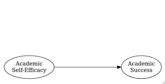
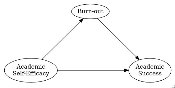
  • E.g., Bulfone et al. (2022)
    • Found that there is a direct effect of academic self-efficacy on academic success
    • And that burn-out mediated part of that relationship
    • (The effects were similar among TWIA males & females)

Causality without Counterfactuals

  • Hill (1965) proposed nine guidelines to help evaluate whether an observed association may be causal
    • N.b., these are not strict rules
      • “What I do not believe … is that we can usefully lay down some hard-and-fast rules of evidence [for] cause and effect.” (p. 299)
  • Offers a practical framework for causal reasoning
    • Esp. where counterfactuals are difficult to study
      • E.g., epidemiology, public & environmental health, policy analysis, etc.

The End