Frequencies,
Counts, &
Distributions
Overview
- Frequencies & relative frequencies
- Probabilities
- Risks & risk ratios
- Hazards & hazard ratios
- Odds & odds ratios
- Contingency / cross tables
- Fisher’s exact test
- Important distributions
- Normal distribution
- χ² distribution
Frequencies
&
Relative Frequencies
Frequencies
- Simply how often something occurs
- But can be expressed differently:
-
Relative to the entire
sample
- “Of all 100 patients, 80 had pain disorders”
- Presented as percents, probabilities, or risks
-
Relative to other
subgroups
- “80 of these patients developed pain disorders, and 20 did not”
- Presented as odds
- “The odds of these patients developing a pain disorder were 4:1”
Relative Frequencies
- We’re often interested not only in how something happens
- But if it’s more/less common in one group/situation than in others
- This is the relative frequency
- Can be expressed as:
- Relative risk (relative probability)
- Relative odds
- These are usually instead written as:
- Risk ratio
- Odds ratio
- Can be expressed as:
Risks
(Probabilities)
& Risk Ratios
Risks/Probabilities
- Again, risk & probability are the same thing
- Expressed as the chance of something happening standardized to a
scale of 0 to 1
- Often computed as the chance—or number of times—something happens out of all possible times
\[P(\mathsf{Target\ outcome}) = \frac{\mathsf{Number\ of\ target\ outcomes}}{\mathsf{Number\ of\ all\ outcomes}}\]
\[P = \frac{72}{200} = .36\]
Risks/Probabilities (cont.)
pain.df <- data.frame(Ethnicity = c("Latin", "Non-Latin"),
                      Diagnosed = c(72, 223),
                      Not_Diagnosed = c(128, 241)
)<-assigns a value, function, etc. to an “object”- Here I’m creating a
data.frame - And assigning it to / saving it as
pain.df
- Here I’m creating a
c“concatenates” (combines) a series of values, etc. into a single list (“array” or “vector”)
Risks/Probabilities (cont.)
library(knitr)
library(kableExtra)
table.of.pain <- pain.df %>%
  kable(col.names = c("Ethnicity", "Diagnosed", "Not Diagnosed"),
        align = c("l", "c", "c")) %>%
  kable_styling(font_size = 42) %>% kable_material("hover") %>%
add_header_above(c(" " = 1, "Pain Disorder Diagnosis" = 2))- Most functions in
Rare available in add-on packages;libraryinvokes a given packageknitrprepares output for reportskableExtraspimps out tables (kables) made byknitr
%>%is a “pipe” command, which essentially nests commands inside other commands- I’m piping commands to tweak the table into the
pain.dfdata frame - And having all of that assigned to the
table.of.painobject
- I’m piping commands to tweak the table into the
Risks/Probabilities (cont.)
- Simply giving the name of an object invokes it
- (Kinda like Satan)
|
Pain Disorder Diagnosis
|
||
|---|---|---|
| Ethnicity | Diagnosed | Not Diagnosed |
| Latin | 72 | 128 |
| Non-Latin | 223 | 241 |
Risks/Probabilities (end)
\[P(\mathsf{Latino\ Patient\ Has\ a\ Pain\ Disorder}) = \frac{\mathsf{Target\ Event}}{\mathsf{All\ Events}}\]
\[= \frac{\mathsf{Latinos\ \overline{c}\ Pain\ Disorders}}{(\mathsf{Latinos\ \overline{c}\ Pain\ Disorders})+(\mathsf{Latinos\ \overline{s}\ Pain\ Disorders})}\]
\[= \frac{72}{72+128} = \frac{72}{200} = .36\]
More Computations with R
- Brackets (
[]) index parts (“elements”) of an object
## [1] "Latin"## [1] 72## Ethnicity Diagnosed Not_Diagnosed
## 1 Latin 72 128More Computations with R (cont.)
##   Ethnicity Diagnosed Not_Diagnosed
## 1     Latin        72           128
## 2 Non-Latin 223 241## [1] 200p.latin.patient.diagnosed.with.pain.disorder <- pain.df[1, 2] / (pain.df[1, 2] + pain.df[1, 3])
p.latin.patient.diagnosed.with.pain.disorder## [1] 0.36More Computations with R (cont.)
$accesses a column (or other variable-like element) of an object…
## [1] "Latin" "Non-Latin"## [1] 72 223More Computations with R (cont.)
- We can do computations etc. on these columns
## [1] 0.3600000 0.4806034More Computations with R (cont.)
- And assign those computations to an element
- That’s also part of that data frame
pain.df$Risk_of_Pain_Diagnosis <- pain.df$Diagnosed /
          (pain.df$Diagnosed + pain.df$Not_Diagnosed)
pain.df$Risk_of_Pain_Diagnosis
## [1] 0.3600000 0.4806034## Ethnicity Diagnosed Not_Diagnosed Risk_of_Pain_Diagnosis
## 1 Latin 72 128 0.3600000
## 2 Non-Latin 223 241 0.4806034More Computations with R (end)
- The risk ratio is simply the ratio of these risks:
\[\mathsf{Risk\ Ratio} = \frac{\mathsf{Risk\ Among\ Latino\ Patients}}{\mathsf{Risk\ Among\ Non\text{-}Latino\ Patients}}\]
\[= \frac{.36}{\sim.48} \approx .75 \]
## [1] 0.7490583Hazards
&
Hazard Ratios
Hazards & Hazard Ratios
- Hazard is simply risk within some time frame
- “What are the risks of relapse within one year?”
- Hazard ratio is the hazard in one group relative to an other
- “What are the risks of Latino patients relapsing within one year compared to non-Latino patients?”

Presentation of Hazards
- Since events in a time frame may not be uniform,
- Hazards / hazard ratios are often accompanied by “Kaplan-Meier curves” depicting events over time

Probability of continued opioid use for ≤ 365 days for patients with
childbirth, surgery, trauma, or other pain diagnosis in the week before
their first opioid prescription or chronic pain diagnosis in the 6
months before their first opioid prescription.
Abbreviation: CNCP,
chronic non-cancer pain
Shah, Hayes, & Martin (2017)
Analyzing Hazards
- Cox proportional hazards regression
- Tests if variables can significantly predict hazard (time-to-event)
- Handles “censoring” well
- When we don’t know how long it was to an event because, e.g., the
event didn’t happen during the study
- (E.g., the patient survived until at least the end of the study window)
- When we don’t know how long it was to an event because, e.g., the
event didn’t happen during the study
- Assumes that the effect of each predictor on the outcome is
consistent throughout the study
- E.g., there is no seasonal effect
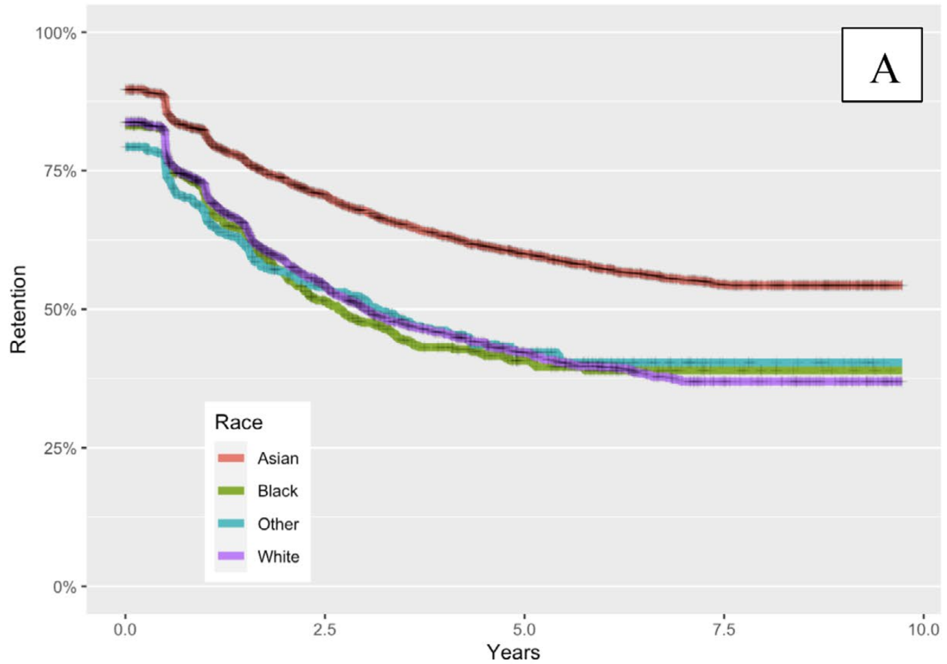
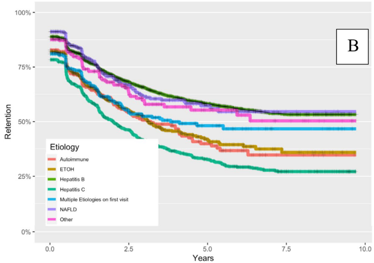
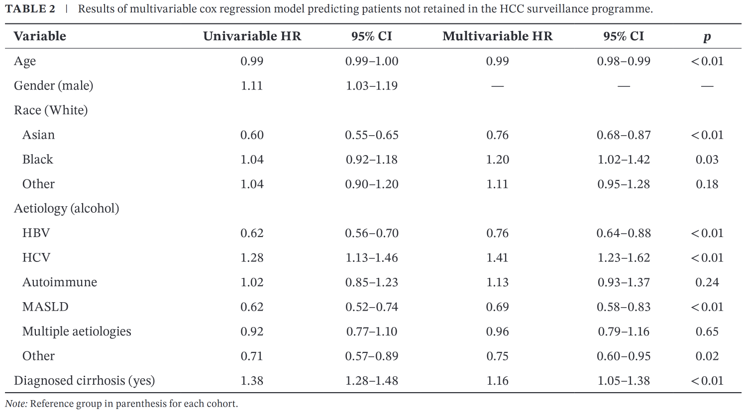
Example of Cox Regression
- Brahmania et al. (2025)
- Investigated the effects of a dedicated, automated recall
hepatocellular carcinoma (HCC) surveillance program on retention
- Among 7,269 Canadian patients with a confirmed diagnosis of cirrhosis of any aetiology
- Who were automatically enrolled in a surveillance program
- Predictors of retention (returning for screenings):
- Patients who identified as Asian were most likely to return for semi-annual screenings (of races)
- Patients diagnosed with Hepatitis B, autoimmune, or alcohol-induced cirrhosis least likely (of aetiologies)
- Investigated the effects of a dedicated, automated recall
hepatocellular carcinoma (HCC) surveillance program on retention
Example of Cox Regression (cont.)
Example of Cox Regression (cont.)
Example of Cox Regression (end)
Odds
&
Odds Ratios
Risks vs. Odds
- Probability is the chance of something happening
out of all possible occasions
- E.g., of the 200 Latino patients with OUDs, 72 were diagnosed with pain disorders
\[P(\mathsf{Being\ Diagnosed\ \overline{c}\ Pain\ Disorder})= \frac{72}{72+128} = \frac{72}{200}\]
- I.e., \(\frac{72}{200} = .36 \approx \frac{1}{3}\) of all Latino patients with OUDs were diagnosed with a pain disorder
- “36% of these Latino patients with OUDs were diagnosed with a pain disorder.”
Risks vs. Odds (cont.)
- Odds are the chance of something happening relative
to them not happening
- E.g., 72 Latino patients were diagnosed with pain disorders
- 128 Latino patients were not so diagnosed
\[\mathsf{Odds\ of\ Being\ Diagnosed\ \overline{c}\ Pain\ Disorder} = \frac{72}{128} \approx .56\]
-
“Among these Latino patients with OUDs,
- For every 1 diagnosed with a pain disorder,
- There were about 2 who were not (odds = 0.56).”
Examples of Odds
| Event Happening | Odds of Event |
|---|---|
| Dying in a plane crash | 1 : 11,000,000 |
| Winning an Olympic medal | 1 : 622,999 |
| Being killed by a meteorite | 1 : 250,000 |
| Dying in a hurricane | 1 : 62,288 |
| Experiencing accidental awareness during general anesthesia | 1 : 19,600 |
| Getting struck by lightning within an 80-year life | 1 : 15,300 |
| Being involved in a mass shooting | 1 : 11,125 |
| Finding a four-leaf clover | 1 : 10,000 |
| Loosing your home to fire | 1 : 3,000 |
| Dying in a motorcycle accident | 1 : 722 |
| Being matched as a bone marrow donor | 1 : 430 |
| Getting your car stolen | 1 : 332 |
| Giving birth on the actual due date | 1 : 249 |
| Being audited by the IRS | 1 : 220 |
| Having an application accepted by Harvard | 1 : 30.25 |
| Identifying as LGBTQ+ | 1 : 16.86 |
| Being an adult with hearing issues | 1 : 6.14 |
| Dying by heart disease | 1 : 6 |
| Being an elderly adult with hearing issues | 1 : 1 |
| Earn any degree within 6 years of enrolling in a 4-year for-profit college | 1 : 1.68 |
| Earn any degree within 6 years of enrolling in a 4-year public college | 1 : 0.52 |
| Being saved by CPR | 1 : 1.44 |
From Stacker
Odds Ratios
- Odds ratios (OR) represent the odds of an event in
one group proportional to the odds in an other
- E.g., OR = .5 means the odds in the target group are half the odds
in the reference group
- E.g., the odds in the target group are 2:1
- While the odds in the reference group are 4:1
- E.g., the odds in the target group are 2:1
- E.g., OR = .5 means the odds in the target group are half the odds
in the reference group
- Turning back to the OUD study may help…
Odds Ratios: Example
| Ethnicity | Diagnosed | Not Diagnosed |
|---|---|---|
| Latin | 72 | 128 |
| Non-Latin | 223 | 241 |
Odds—not odds ratios—for each group:
- Odds of pain diagnosis among Latino patients with OUDs: \(\frac{N_{\mathsf{Latinos\ \overline{c}\ Pain\ Disorders}}}{N_{\mathsf{Latinos\ \overline{s}\ Pain\ Disorders}}} = \frac{72}{128} \approx .56\)
- Odds of pain diagnosis among non-Latino patients with OUDs: \(\frac{N_{\mathsf{non-Latinos\ \overline{c}\ Pain\ Disorders}}}{N_{\mathsf{non-Latinos\ \overline{s}\ Pain\ Disorders}}} = \frac{223}{241} \approx .92\)
Odds Ratios: Equation
| Group | Present | Not Present) |
|---|---|---|
| Target | A | B |
| Reference | C | D |
\[OR = \frac{(\textsf{Target & Present / Target & Not Present})}{(\textsf{Reference & Present / Reference & Not Present})}\]
\[OR = \frac{(\textsf{A / B)}}{\textsf{(C / D)}}\]
Odds Ratios: Example (cont.)
| Ethnicity | Diagnosed | Not Diagnosed |
|---|---|---|
| Latin | 72 | 128 |
| Non-Latin | 223 | 241 |
\[OR = \frac{(\textsf{Latin & Diagnosed / Latin & Not Diagnosed})}{(\textsf{Non-Latin & Diagnosed / Non-Latin & Not Diagnosed})}\]
\[OR = \frac{(72 / 128)}{(223 / 241)} \approx \frac{.56}{.92}\approx .61\]
- The odds of a Latino patient being diagnosed with a pain disorder were about 61% of the odds for a non-Latino patient.
Odds Ratios: Example (cont.)
- Could also look at it from the non-Latin perspective
\[OR = \frac{(223 / 241)}{(72 / 128)} = \frac{.92}{.56} \approx 1.6\]
Note that \(\frac{1}{.61} \approx 1.6\)
- For every 1 Latino OUD patient diagnosed with a pain disorder, 1.6 Non-Latino OUD patients are so diagnosed
Contingency
Tables &
Fisher’s Exact Test
Contingency Tables
- Also called “cross tables”
- Displays the counts (frequencies) of events in different categories
- And often used to compute probabilities
- Is usually intended to be used when outcomes are “exclusive”—that all options are presented
- IFF it is exclusive, can
conduct meaningful tests on whether the frequencies differ between
groups, etc.
- Fisher’s
exact test can be used to test 2 \(\times\) 2 tables
- N.b., Fisher’s exact test can also be used on contingency tables larger than 2 \(\times\) 2
- In fact, it’s better than χ² with small cell counts (<5)
- Fisher’s
exact test can be used to test 2 \(\times\) 2 tables
Contingency Tables (cont.)
Yeah, like this:
| Ethnicity | Diagnosed | Not Diagnosed |
|---|---|---|
| Latin | 72 | 128 |
| Non-Latin | 223 | 241 |
- Odds among Latinos = \(\frac{72}{128} \approx .56\)
- Odds among non-Latinos = \(\frac{223}{241} \approx .92\)
- Odds ratio = \(\frac{.56}{.92} \approx .61\)
Fisher’s Exact Test
- Invented to test if Fisher’s colleague, Muriel Bristol, could indeed tell if cream or tea were poured first into a cup
- Called an “exact” test because it computes the exact
p-value for rejection
- I.e., not an estimate based on
inferences about the population
(e.g., normality) - So, isn’t inferential per se
- I.e., not an estimate based on

waiting for her tea
Fisher’s Exact Test Example
pain.df.counts <- subset(pain.df, select = c("Diagnosed", "Not_Diagnosed"))
fisher.test(pain.df.counts)
##
## Fisher's Exact Test for Count Data
##
## data: pain.df.counts
## p-value = 0.00491
## alternative hypothesis: true odds ratio is not equal to 1
## 95 percent confidence interval:
## 0.4250886 0.8665430
## sample estimates:
## odds ratio
## 0.6083658- The difference in odds (0.56 vs. 0.92) is significant at α = .05
- We see this in
p-value = 0.00491 - And that the confidence interval (
0.425–0.866) for the odds ratio (0.608) doesn’t overlap 1
- We see this in
Fisher’s Exact Test Example (cont.)
fisher.testalso creates an object- And not all elements of that object are automatically printed
- We can look to see what all is there with either the powerful &
flexible
summary()command:
##             Length Class  Mode
## p.value     1      -none- numeric
## conf.int    2      -none- numeric
## estimate    1      -none- numeric
## null.value  1      -none- numeric
## alternative 1      -none- character
## method      1      -none- character
## data.name   1      -none- character
Fisher’s Exact Test Example (cont.)
- Or with the more revealing
str()command:str()works to “look inside” most any object or function inR
## List of 7
##  $ p.value    : num 0.00491
##  $ conf.int   : num [1:2] 0.425 0.867
##   ..- attr(*, "conf.level")= num 0.95
##  $ estimate   : Named num 0.608
##   ..- attr(*, "names")= chr "odds ratio"
##  $ null.value : Named num 1
##   ..- attr(*, "names")= chr "odds ratio"
##  $ alternative: chr "two.sided"
##  $ method     : chr "Fisher's Exact Test for Count Data"
##  $ data.name  : chr "pain.df.counts"
##  - attr(*, "class")= chr "htest"
Fisher’s Exact Test Example (cont.)
$can access any of those elements of thefisher.testobject:
## [1] 0.004910079## [1] 0.4250886 0.8665430
## attr(,"conf.level")
## [1] 0.95Is Fisher’s Exact Test Too Conservative?
- Fisher himself sure was
- Fisher’s exact test can mis-estimate p-values when the
total N is “small” (<50; Andrés & Tejedor, 1995)
- But this bias itself is usually small
- And common corrections (e.g., Yate’s
correction) don’t change outcomes much (Crans & Shuster, 2008)
- While making for somewhat more complicated analyses that rely on parametric assumptions
Upton (1992)
- Upton (1992)
argues that Fisher’s exact test is not too conservative
- Trouble comes because counts are discrete
- While p-values assume the data are continuous
- Trouble comes because counts are discrete
- Also discusses how it can be hard to test this when something comes
close to always (or never) happening
- Essentially, cell counts that are zero (or close to it) can be problematic
- And that small cell counts can push a p-value to be larger
than .05
- See Upton’s discussion of Table 2 where the real rejection value ranged from .015 – .080
Upton (1992, cont.)
- Also notes—correctly—that significance is largely determined by
sample size
- Some argue for making α smaller as samples get larger
- Can add confidence intervals (CIs) to the concomitant OR
- (And perhaps p-values for the ORs at the CI limits)
- Or even use Bayesian inferences
- Discussed “practical significance”
- I.e., how important it is to not have false positives for a given real-world situation
- “The experimenter must keep in mind that significance at the 5% level will only coincide with practical significance by chance!” (p. 397)
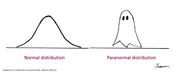
The Normal Distribution
Normal Distribution
Formula for a normal distribution:
\[f(x, \mu, \sigma) = \frac{1}{\sigma\sqrt{2\pi}}e^{\frac{-(x - \mu)^2}{2\sigma^2}}\]
- x is some random variable
- μ is the mean
- σ is the standard deviation
- There, now you can say you learned this
Characteristics

Characteristics (cont.)
- Most importantly, it is only a function of the mean & standard deviation
- The mean, median and mode are all equal
- The total area under the curve equals 1
- It’s symmetric
- The curve approaches—but never touches—the x-axis
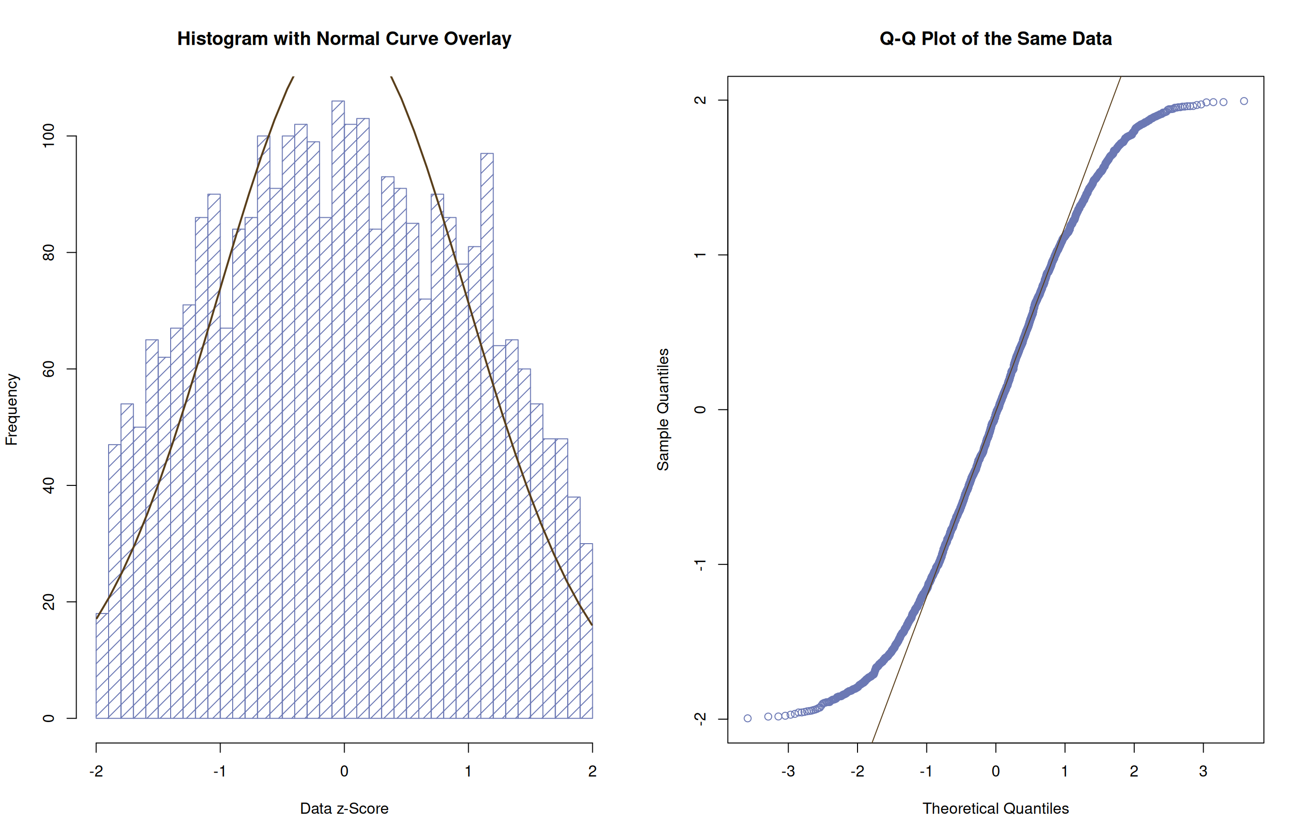
Q-Q Plots
- “Quantile-quantile” plots
- Compare the position in the distribution of a given quantity against the position of the same quantity in an other (e.g., normal) distribution
- More simply, how & where two distributions deviate from each other
- Frequently used to test if & how a sample deviates from
normality
- Or how residuals deviate from normality
- They’re easily created in SPSS
or R
- They can be done—less easily—in Excel, etc
- And a few examples may help understand them…
Normally-Distributed

Short Tails (Looks like an S )
Long Tails

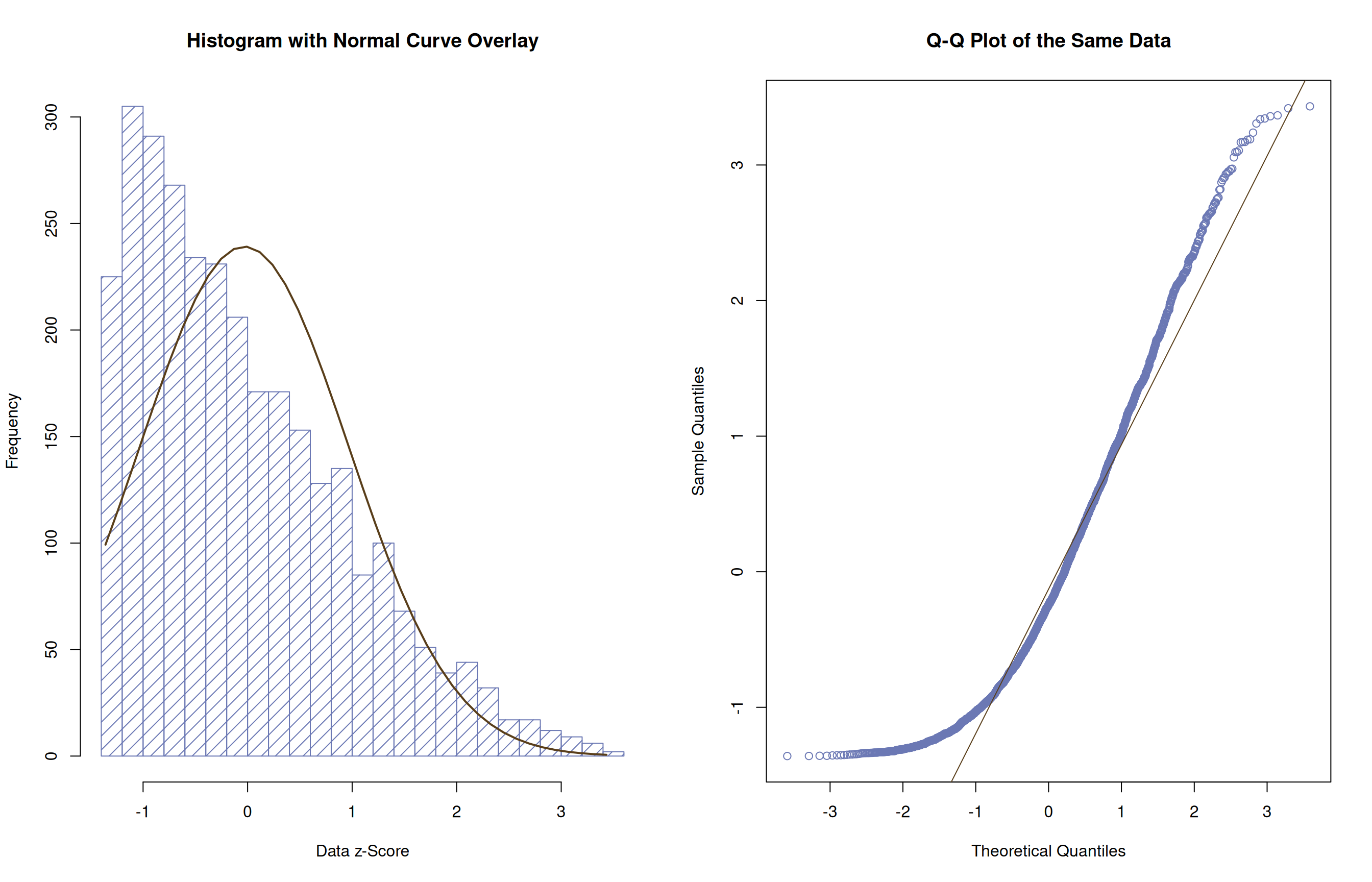
Long Right Tail (Positive Skew)
Long Left Tail (Negative Skew)

More Figures, More Views on Skew
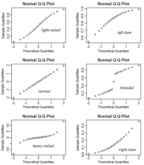
From StackExchange
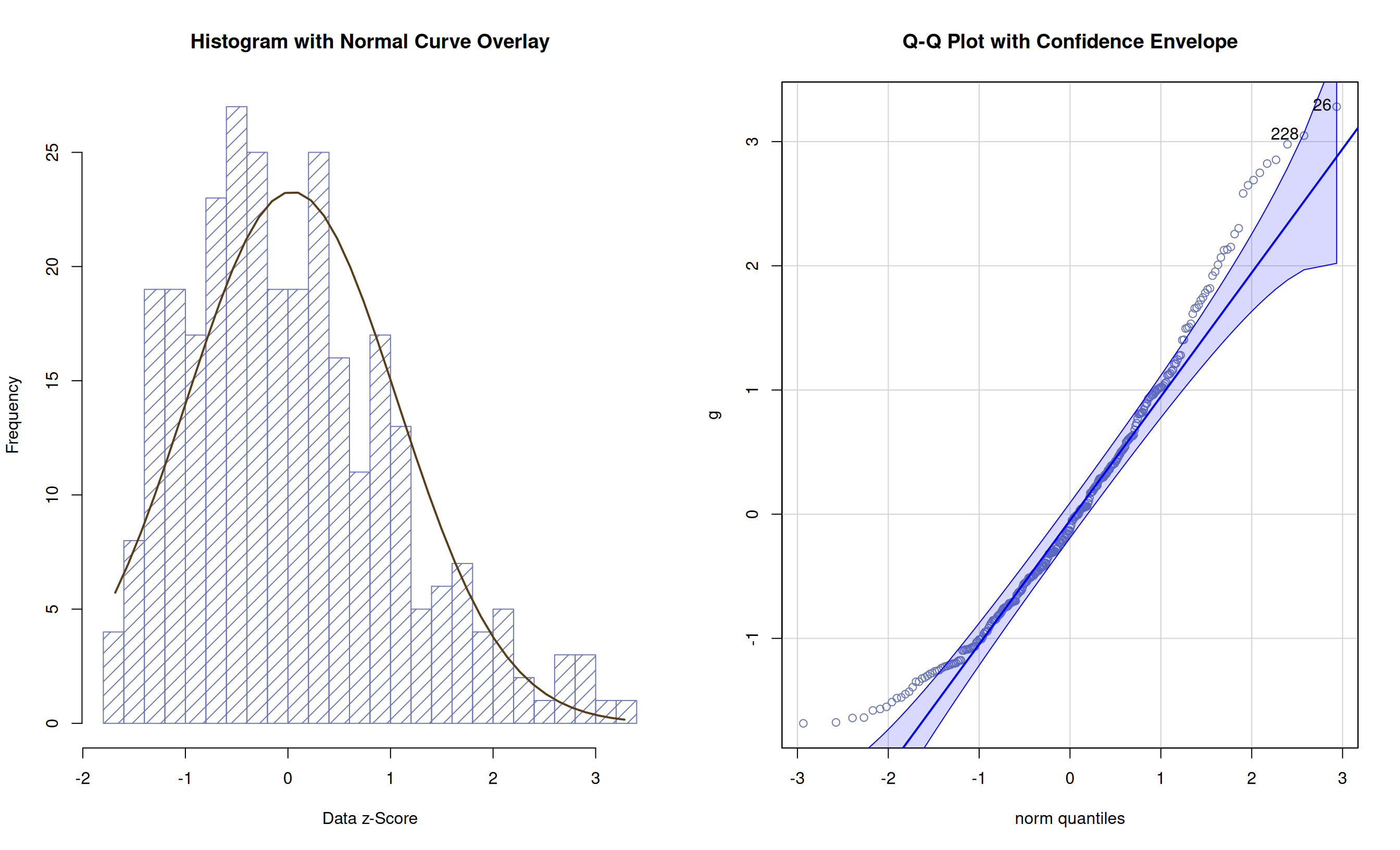
Q-Q Plots (cont.)
- Can put a “confidence envelope” around data in Q-Q plots:
Alternatives to Q-Q Plots
- Can also/instead formally test normality of a sample with, e.g.:
- S-W
and A-D are better than K-S, but all are strongly affected by sample
size
- Under-powered with small N
- Can’t detect non-normality when we need to
- Over-powered with large N
- Overly sensitive to deviations when we don’t need to know
- (I.e., have enough data to approximate population distribution without assuming normality)
- Under-powered with small N
The χ² Distribution
Background
- Invented by Karl Pearson (in an abstruse 1900 article)
- Originally to test “goodness
of fit”
- I.e., how well a set of data fit a theoretical distribution
- Or if two sets of data follow the same distribution
- Technically, χ² is a type
of Gamma
distribution created by the distribution of sums of the squares of a
set of standard normal random variables
- A lot like we get when computing ordinary least squares for t-tests & ANOVAs
- And is closely related to the t and F distributions
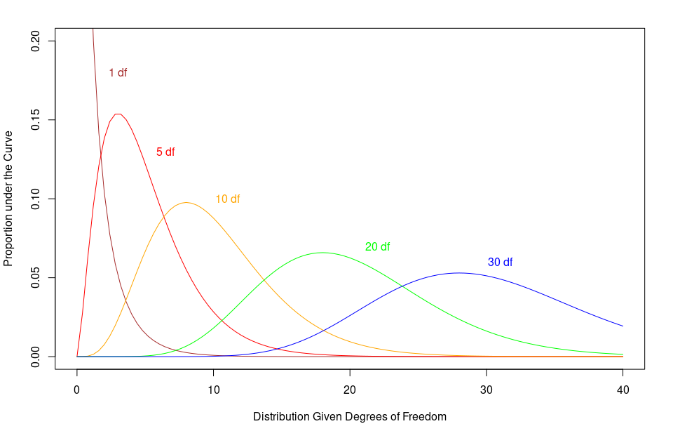
Characteristics
- The distribution’s shape, location, etc. are all determined by the
degrees of freedom
- The mean = df
- The variance = 2df
- SD = \(\sqrt{2df}\)
- The maximum value for the y-axis = df – 2
(when dfs >1)
- As the degrees of freedom increase:
- The χ² curve approaches a normal distribution
- The curve becomes more symmetrical
- It has no negative values
- Since it is based on squared values
- Making it good to test variances
Characteristics (cont.)
Computing χ²
Formula for χ² value:
\[\chi^2 = \sum{\frac{(\mathsf{Observed} - \mathsf{Expected})^2}{\mathsf{Expected}}}\]
- Compute the differences between a data’s actual value from it’s expected value
- Square all of those differences & divide by the expected value
• Kinda like computing the odds - Sum up those square differences “odds” for each group
- Check that summed value against a χ² distribution
• Where dfs = (Nrows – 1) \(\times\) (Ncolumns – 1) - If the summed value is really far from the center of the
distribution
• Then those actual-expected differences are significant
Example of Using χ²
- Remember our data for Latino patients with OUDs:
| Ethnicity | Diagnosed | Not Diagnosed | Total |
|---|---|---|---|
| Latin | 72 | 128 | 200 |
- Presenting that a little differently:
| Value Type | Diagnosed | Not Diagnosed | Total |
|---|---|---|---|
| Observed | 72 | 128 | 200 |
| Expected | 100 | 100 | 200 |
Example of Using χ² (cont.)
- Taking the difference between observed & expected
- Squaring those differences & dividing by expected
- Add up those values
| Value Type | Diagnosed | Not Diagnosed |
|---|---|---|
| Observed | 72 | 128 |
| Expected | 100 | 100 |
| Observed – Expected | -28 | 28 |
- \(28^2 = 784\) (and -\(28^2 = 784\))
- \(\frac{784}{100} = 7.84\)
- \(7.84 + 7.84 = 15.68\)
- df = \((2 - 1)\times(2 - 1) = 1\times1 = 1\)
Example of Using χ² (end)
- The critical χ² value
- For 1 df
- And α = .05:
- (
lower.tail = FALSEgives the max value for a χ² from the null distribution)
## [1] 3.841459- Which is smaller than our χ² of 15.68
- So our observed values are significantly different than our expected ones
Uses of χ²
- Because it only depends on df,
- And resembles a normal distribution.
- It is useful for testing if data follow a normal distribution
- Or often if the total set of deviations from normality
- (Or any set of expected values)
- Are greater than expected
- Or often if the total set of deviations from normality
- It can do this for discrete values—like counts
- t and F distributions technically can’t do this
Uses of χ² (cont.)
- The χ² distribution has many
uses, including:
- Estimating of parameters of a population of an unknown distribution
- Checking the relationships between categorical variables
- Checking independence of two criteria of classification of multiple qualitative variables
- Testing deviations of differences between expected and observed frequencies
- Conducting goodness of fit tests
Example of a χ² Test
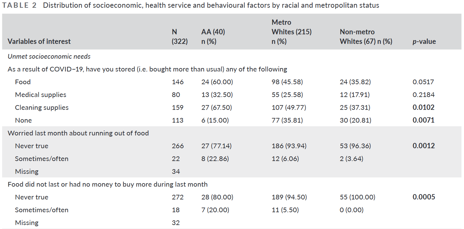
Notes: “AA” = African Americans; p-values are from tests of χ²s
Zhang, A. Y., Koroukian, S., Owusu, C., Moore, S. E., & Gairola, R. (2022). Socioeconomic correlates of health outcomes and mental health disparity in a sample of cancer patients during the COVID-19 pandemic. Journal of Clinical Nursing. https://doi.org/10.1111/jocn.16266