Exploring Correlations and Partial Correlations in the Midlife in the United States Study

1 Objectives

1. To investigate and report upon correlations and partial correlations
2. To conduct and report upon an ANCOVA upon a similar set of variables

2 Background

The Midlife in the United States (MIDUS) study is a national longitudinal research project examining how psychological, social, and biological factors affect health and aging. It began in 1995–96 with over 7,000 adults aged 25–74 and has continued through multiple follow-up waves. MIDUS includes survey data, daily diaries, cognitive testing, and biological samples.

In 2012, MIDUS added a Milwaukee-based sample of about 500 African American adults as part of its “refresher wave.” This oversample was designed to address racial disparities and increase the study’s diversity. It focused on factors like socioeconomic status, discrimination, health, family life, and spirituality, aiming to explore how stress, race, and culture intersect to affect well-being.

Data are publicly available through ICPSR and the MIDUS website, and the study has supported extensive research on health disparities, resilience, and aging. The data included here are a subset of the full set of over 2,000 variables.

2.1 Data

The data are available in Brightspace in two formats:

• As an SPSS data file.
  • The variable labels are taken from the descriptions given in both the official MIDUS Codebook and the one created for our subset of variables.
• As a CSV file.
  • Do please refer to this codebook for explanations of the variables.

I have created a sort of codebook for the subset of variables we will use. That codebook includes links to the actual, official MIDUS Codebook that explains what each of the variables in this subset measure. You will see that many of the variables are coded so that higher scores are less desirable (denoting worse health, etc.), so please do be mindful of this when interpreting the results.

Please also note that these data are made available to you for use in this course only. For any other uses, including in published research, one must register with the MIDUS study.

3 Investigating the Relationships

You may use either Excel/Calc or SPSS (e.g., via Apporto) to compete this assignment. Note, however, that it is much easier to compute partial correlations in SPSS.

Whichever you choose to use, please:

1. Choose 5 – 10 variables you find the most interesting.
2. Present the correlations between them in a correlation matrix (either a full or, e.g., just the lower triangular diagonal).
3. Choose two bivariate correlations¹ (between two different sets of variables²); present both of these two correlations along with partial correlations between these same pairs. You may use the same, third variable to partial out of these bivariate correlations or a different third variable for each bivariate.
4. Interpret all of these results as they could be presented in a Results section of a manuscript.

Your deliverable will be a Word/Writer or PDF document that presents the tables/figures and text as they would in a typical (e.g., APA-formatted) Results section.

4 Conducting Correlations and Partial Correlations

4.1 In Excel

4.1.1 Creating Correlations

The process is, of course, the same as was done in the previous assignment:

1. Choose the Data ribbon in Excel

2. Click on Data Analysis under the Analyze section of that ribbon

3. In the dialogue box that opens, select Correlation and then OK.

4. In the next dialogue box that opens, click the small icon next to the Input Range field to minimize that dialogue: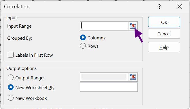

   

5. Select the range of cells that contains the two columns you’d like to correlate³. It’s all right that your selection will include more columns than just those two.

6. Once you’ve selected the cell range you’d like to correlate, click on the little icon to the right of the Input Range field again to expand out that dialogue box:

   

7. Back in that dialogue box:

   1. Leave selected Group By: Columns
   2. Select Labels in First Row
   3. Under the Output options section, select New Worksheet Ply and give that new worksheet a name, e.g., Correlation⁴.

4.1.2 Creating Partial Correlations

This is not as easy to do in Excel.

1. Choose which two variables you would like to correlate and which third variable you would like to partial out of that correlation. Let us say you are using RAACA2, RAACA1, RAACAS6A, which are, respectively:
   • Mental/emotional health self-evaluated
   • Physical health self-evaluated
   • Compare energy now to 5 years ago
2. Regress RAACA2 on RAACAS6A and get residuals
   1. Go to Data > Data Analysis > Regression (first enabling the Analysis Toolpak if needed).
      
   2. Set RAACA1 Range = RAACA2, RAACA2 Range = RAACAS6A.
      
   3. Check Output Residuals and run the regression.
      
   4. Save the residuals for RAACA2 (call them, say, A1_AS6A) in, e.g., column BP.
3. Regress RAACA1 on RAACAS6A and get residuals
   1. Repeat the regression, this time with RAACA1 as the dependent variable and RAACAS6A as the independent variable.
      
   2. Save the residuals for RAACA1 (call them, say, A1_AS6A) in column BQ.
4. Correlate the residuals
   1. Use the CORREL function to calculate the correlation between RX and RY:
      =CORREL(BP3:BP510, BQ3:BQ510)
   2. This value is the partial correlation between RAACA2 and RAACA1, controlling for RAACAS6A.

4.2 In SPSS

4.2.1 Creating Correlations

1. Click on Analyis > Correlate > Bivariate ...
2. In the dialogue box that opens, add the variables you would like to correlate to the Variables field
3. In the Correlation Coefficients section of that dialogue, leave Pearson checked (since there are variables that are certainly interval/ratio)
   • Many of the variables are from Likert-scaled items. Some argue to treat these like ordinal variables, in which case you could select to also include either Kendall's tau-b or Spearman. As we noted in lecture, Kendall’s \(\tau\) is less efficient than Spearman’s \(\rho\). Spearman’s \(\rho\) is efficient enough that it tends to produce results similar to Pearson’s r while also being more robust than r.
   • So, if you want to use either of these, I suggest selecting Spearman.
4. In the Test of Significance section, leave Two-tailed checked. As we also noted in lecture, two-tailed tests evaluate whether the correlation is different than zero in either direction (positive or negative). (A one-tailed would evaluate if the correlation is only, e.g., both different from zero and positive.)
   • Also leave checked to Flag significant correlations to let SPSS place asterisks next to correlations where p < .05 etc.
   • You can also select to Show only the lower triangle of the correlation (and then perhaps de-select Show diagonal to remove the auto-correlations that are all 1s). This will only show the bottom half of the correlation matrix. Some prefer this since style; it’s your choice if you do, too.
5. Click on the Options button; in the dialogue that opens, choose Exclude cases pairwise—not the default option for SPSS, Exclude cases listwise⁵.
   • You can also ask SPSS to present to Means and standard deviations if you want. Presenting the Cross-product deviations and covariances would show the unstandardized associations between the variables, which doesn’t really add anything here.
6. In the Confidence interval... dialogue, you can also select to Estimate confidence interval of bivariate correlaiton parameter, leaving the Confidence interval (%) to be 95 (reflecting \(\alpha\) = .05).
   • If you choose to add Spearman’s \(\rho\), then it doesn’t hurt to also Apply the bias adjustment. Spearman’s \(\rho\) can mis-estimate correlations with small samples (usually n < 30); this adjustment helps offset that bias. Our sample size is large enough that this shouldn’t matter, but this adjustment wouldn’t adversely affect large correlations.
7. Click OKs to finish and marvel at your work.

4.2.2 Creating Partial Correlations

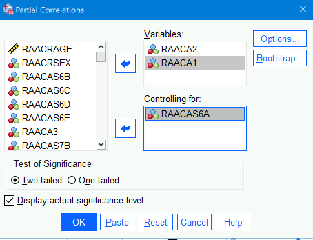
1. Click on Analyis > Correlate > Partial...

2. In the dialogue box that opens:

   1. Add RAACA2 and RAACA2 to the Variables field
   2. Add RAACAS6A to the Contorlling for field:

   ::: {.cell} ::: {.cell-output-display} ::: :::

   • Note that under the Options button, you can choose to present either Means and standard deviations to present those or Zero-order correlations to present the bivariate (aka “zero-order”) correlations along with the partial correlations.
   • Please also choose to Exclude cases pairwise.

3. Click OK.

This will report the bivariate correlation between RAACA2 (Mental/emotional health self-evaluated scaled where higher numbers denote worse health) and RAACA1 (Physical health self-evaluated, scaled the same), controlling for RAACAS6A (Compare energy now to 5 years ago).

This could be described as:

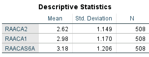
Table 1 presents the mean, standard deviation, and number of responses to RAACA2 (Mental/emotional health self-evaluated) and RAACA1 (Physical health self-evaluated) and RAACAS6A (Compare energy now to 5 years ago). All variables were coded so that higher values denote worse outcomes. For RAACA2 and RAACA1, values ranged from 1 (“Excellent”) to 5 (“Poor”); “Don’t know” and refusals to respond were coded as missing values.

Table 1: Mean, SD, and N Self-Reported Mental/Emotional Health (RAACA2), Physical Health (RAACA1), and Whether One’s Energy Has Improved or Worsened Compared to 5 Years Ago.

We can see in Table 1 that participants tended to self-report slightly better mental than physical health (\(\overline{X}_{Mental}\) = 2.62; \(\overline{X}_{Physical}\) = 2.98; lower values denote better health). Most participants reported that their health was getting slightly worse (\(\overline{X}\) = 3.18 where 3 = “Stayed the same” and 4 = “Gotten a little worse”.

Table 2: Zero-order Correlation Between Self-Reported Mental/Emotional Health (RAACA2) and Physical Health (RAACA1) Along with the First-Order Controlling for Whether One’s Energy Has Improved or Worsened Compared to 5 Years Ago. Significance (2-tailed) presents the p-value for tests of significance.

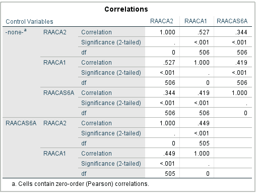
Self-reported mental/emotional health and physical health were strongly and significantly correlated (r = .53, p < .001): feeling better (or worse) about one’s mental health was associated Mental and physical health tended to move the same direction. This relationship was in part due to their shared variance with how much energy participants reported having now compared to 5 years ago (partial r = .45); those who felt their health has improved tended to also say that both their mental and physical health were also good.

5 Conducting an ANCOVA

An ANCOVA is an analysis of covariance. It is similar to other ANOVAs in that it compares the mean of a continuous outcome across groups, but it also controls for one or more continuous covariates. In other words, ANCOVA lets you ask whether groups differ on an outcome after statistically adjusting for another variable.

For this section, please choose:

1. One continuous dependent variable
2. One categorical (or—to increase the number of options—an ordinal variable) grouping variable
3. One continuous variable to serve as a covariate

For example, using the MIDUS data, you might test whether body mass index differs across self-rated mental/emotional health groups while controlling for age:

• Dependent variable: RAACBMI (Body mass index)
• Fixed factor/grouping variable: RAACA2 (Mental/emotional health self-evaluated)
• Covariate: RAACRAGE (Age)

Please remember that many of the MIDUS variables are coded such that higher values reflect less desirable outcomes. For RAACA2, higher values indicate worse self-rated mental/emotional health.

5.1 In SPSS

5.1.1 Checking the Homogeneity of Regression Slopes Assumption

ANCOVA assumes that the relationship between the covariate and the dependent variable is approximately the same across groups. In this example, that means that the relationship between age and BMI should be similar across the RAACA2 groups.

To check this assumption in SPSS:

1. Click on Analyze > General Linear Model > Univariate...
2. Add the dependent variable, e.g., RAACBMI, to the Dependent Variable field.
3. Add the categorical predictor, e.g., RAACA2, to the Fixed Factor(s) field.
4. Add the covariate, e.g., RAACRAGE, to the Covariate(s) field.
5. Click on Model....
6. Choose Custom.
7. Add the following terms to the model:
   • RAACA2
   • RAACRAGE
   • RAACA2 * RAACRAGE
8. Click Continue.
9. Click Options....
10. Select:
    • Descriptive statistics
    • Estimates of effect size
    • Homogeneity tests
    • Parameter estimates
11. Click Continue.
12. Click OK.

The key test in this first model is the interaction between the grouping variable and the covariate, e.g., RAACA2 * RAACRAGE. If this interaction is statistically significant, then the relationship between age and BMI differs across mental/emotional health groups. That would mean the standard ANCOVA model is probably not appropriate, at least not without reporting and interpreting that interaction.

If this interaction is not statistically significant, you may proceed with the usual ANCOVA model without the interaction term.

5.1.2 Running the ANCOVA

To run the main ANCOVA model in SPSS:

1. Click on Analyze > General Linear Model > Univariate...
2. Add the dependent variable, e.g., RAACBMI, to the Dependent Variable field.
3. Add the categorical predictor, e.g., RAACA2, to the Fixed Factor(s) field.
4. Add the covariate, e.g., RAACRAGE, to the Covariate(s) field.
5. Click on Model....
6. Choose Custom.
7. Add only the main effects to the model:
   • RAACA2
   • RAACRAGE
8. Click Continue.
9. Click Options....
10. Select:
    • Descriptive statistics
    • Estimates of effect size
    • Homogeneity tests
    • Parameter estimates
11. Move your grouping variable, e.g., RAACA2, into the Display Means for box.
12. Check Compare main effects.
13. Select a correction such as Bonferroni or Sidak.
14. Click Continue.
15. Click OK.

The main output to report is the Tests of Between-Subjects Effects table. In that table:

• The row for the covariate, e.g., RAACRAGE, tells you whether age is significantly related to BMI.
• The row for the grouping variable, e.g., RAACA2, tells you whether adjusted BMI differs across mental/emotional health groups after controlling for age.
• The Partial Eta Squared column gives an effect size for each predictor.

The Estimated Marginal Means table gives the adjusted group means. These are the means for each group after controlling for the covariate.

This could be described as:

An ANCOVA was conducted to examine whether BMI differed across self-rated mental/emotional health groups while controlling for age. The homogeneity of regression slopes assumption was first evaluated by testing the interaction between mental/emotional health and age. If the interaction was not statistically significant, it was removed from the final ANCOVA model. In the final model, age was included as a covariate and self-rated mental/emotional health was included as the grouping variable. Adjusted means were inspected to determine the direction of group differences.

5.2 Using the Online ANCOVA Calculator

You may also compute an ANCOVA using the StatsCalculators ANCOVA calculator.

1. Open the ANCOVA calculator.
2. In the Load Your Data section, either:
   • click Upload Data and upload midus.csv, or
   • open midus.csv, copy the relevant columns, and paste them into the data area.
3. In the Select Columns & Options section, choose:
   • Factor Column: the grouping variable, e.g., RAACA2
   • Covariate Column: the covariate, e.g., RAACRAGE
   • Dependent Variable Column: the outcome, e.g., RAACBMI
4. Leave Sum of Squares Type set to Type II unless you have a specific reason to use another option.
5. Leave the Significance Level set to .05.
6. Click Run ANCOVA Analysis.

In the output, look for:

• The ANCOVA table, especially the row for your grouping variable.
• The adjusted means for each group.
• The assumption checks, especially the test of homogeneity of regression slopes.
• The effect size, usually reported as partial eta squared.

Please note that this calculator can produce post-hoc comparisons as part of the ANCOVA output. These are the most appropriate post-hoc comparisons for the adjusted means because they are based on the ANCOVA model.

5.3 Supplemental Post-Hoc Analyses with Games-Howell

You may also use the Games-Howell post-hoc calculator to examine which groups differ from each other on one of your continuous variables.

However, please note an important distinction: Games-Howell is a post-hoc test for comparing unadjusted group means. It does not control for a covariate. So, if your main analysis is an ANCOVA, Games-Howell should be described as a supplemental follow-up comparison rather than as the adjusted ANCOVA post-hoc test.

For example, you could use Games-Howell to compare mean BMI across levels of self-rated mental/emotional health:

• Grouping variable: RAACA2
• Outcome variable: RAACBMI

To run this test:

1. Open the Games-Howell test calculator.
2. In the Load Your Data section, either upload midus.csv or paste in the relevant columns.
3. In the Select Data Format & Options section, choose Long Format (One row per observation).
4. Set the group column to your grouping variable, e.g., RAACA2.
5. Set the value column to your continuous outcome, e.g., RAACBMI.
6. Leave the significance level set to .05.
7. Click Run Games-Howell Test.

In the output, look for the pairwise comparisons table. Each row compares two groups. Report:

• the two groups being compared
• the mean difference
• the confidence interval
• the adjusted p-value
• whether the groups differ significantly

This could be described as:

Because the grouping variable contained more than two groups, supplemental pairwise comparisons were conducted using Games-Howell tests. Games-Howell was used because it does not require equal variances or equal sample sizes across groups. These comparisons were interpreted as unadjusted follow-up tests and not as a substitute for the adjusted ANCOVA results.

6 Exporting Tables & Figures from SPSS into a Word Processor

If you are using a local version of SPSS (e.g., that you purchased yourself) you can simply right-click on tables and figures to copy them and then paste them into, e.g., MS Word.

However, if you are using SPSS through Apporto, it is less straight forward.

6.0.0.1 Option 1: Work within Apporto

1. Right-click to copy a figure or table within Apporto
2. Open a document in Word within Apporto
3. Paste the figure/table into that online Word document
4. Save that Word document
5. In the Apporto menu at the top of the browser window, click on the Download button:
   
6. In the dialogue that opens, select that Word document to download it to your computer

6.0.0.2 Option 2: Download First from Apporto

Note that it is difficult to modify figures that are exported with these steps, so I advise first making any changes to those within SPSS in Apporto before downloading them.

1. In the SPSS Output window, selection File > Export...
2. In the dialogue that opens:
   1. Select All from the Objected to Export⁶
   2. Under Type, select Word Document (*.docx). Note that several of the other options (e.g., HTML (*.html) or PowerP{oint (*.ppt)) could also work for other uses.
   3. Under File Name, you may change the name of the output file. Note that you should only change the last part of what is presented, after Documents/. Simiarly, I suggest not Browsing to a new location; just leave that going to the default location, which is the Documents folder online.
   4. If you leave the File Name as the default given, you may need to retype that in a Save File dialogue that opens.
   5. Click OK. A Word file that is the exported output file will now be created within Apporto.
3. Click on Download in the Apporto menu at the top of the browser window, and download that output file turned Word document to your computer.
4. You may now open that file on your computer.

Thanks!

Footnotes

1. “Bivaraite correlations” are correlations between two (“bi”) variables. I.e., these are the normal correlations you are used to. (They’re also called zero-order correlations.)

2. I.e., four variables total for bivariate correlations.

3. Using keys, you can move into cell C1, then type Shift + Control/Command + Down Arrow, then—still holding down just the Shift key, tap the Right Arrow key to select over to cell F5017.

4. Since we’re only computing a few correlations, you could also instead choose Output Range and place the correlation somewhere on that same worksheet, e.g., cell J1, but I make it a habit of putting results, new tables, etc. in new worksheets to keep my data in one, clean sheet and any work on it in other sheets.

5. “Excluding cases pairwise” means that if any of the variables used in that particular analysis has a missing value, then skip that row for that analysis. “Excluding cases listwise” means to not include a row of the data if any of the values are missing, regardless of whether they were used in a particular analysis. Listwise deletion, therefore, excludes more data than pairwise. Researchers have found that listwise is often not only too aggressive: it either removes useful information of data are indeed missing as random or accentuates bias if the data are not missing at random.

6. You can select, e.g., All visible, but simplest is just to export the whole output file and then work with it locally.