The
Flexibility of
Linear Models
Linear Models vs. ANOVAs
- ANOVA (and ANCOVA, MANOVA, etc.)
- Is a type of linear regression
- Results focus on significance of variables
- When all are present in the model together
- Linear Regression
- Is a more flexible framework
- Can model complex relationships & data structures
- E.g., non-linear relationships & nested data
- Can test whole models
- And effects on the whole model when variables are added or
removed
Questions Best Addressed by ANOVAs vs. Linear Models
- ANOVAs (and ANCOVAs, MANOVAs, etc.) can ask:
- Which variable is significant?
- Is there an interaction between variables?
- Linear regressions can also ask:
- What is the best combination of variables?
- Does a given variable—or set of variables—significantly contribute
to what we already know?
Signal-to-Noise in Linear
Models
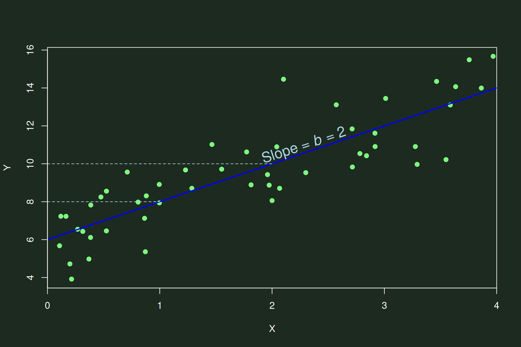
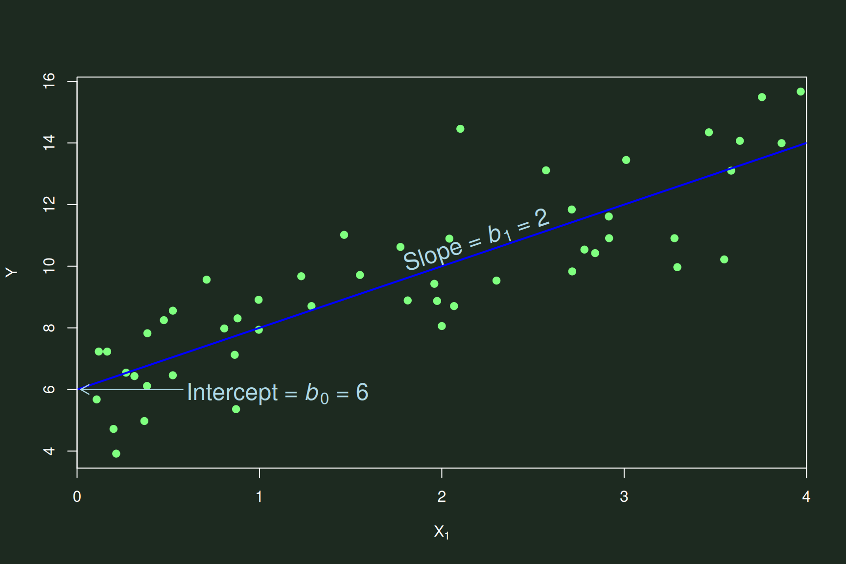
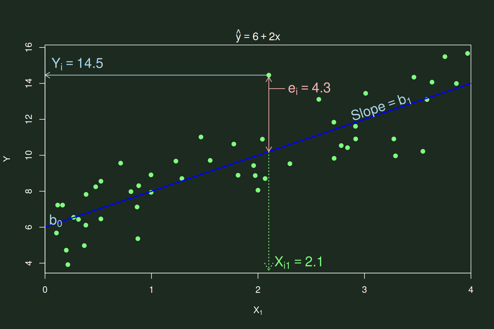
\({Y}_{i} = b_{0} + b_{1}X_{i1} +
e_{i}\)
- The value of \(Y_i\) is partitioned
into:
- That which was predicted by the model: \(b_{0}\) & \(b_{1}\)
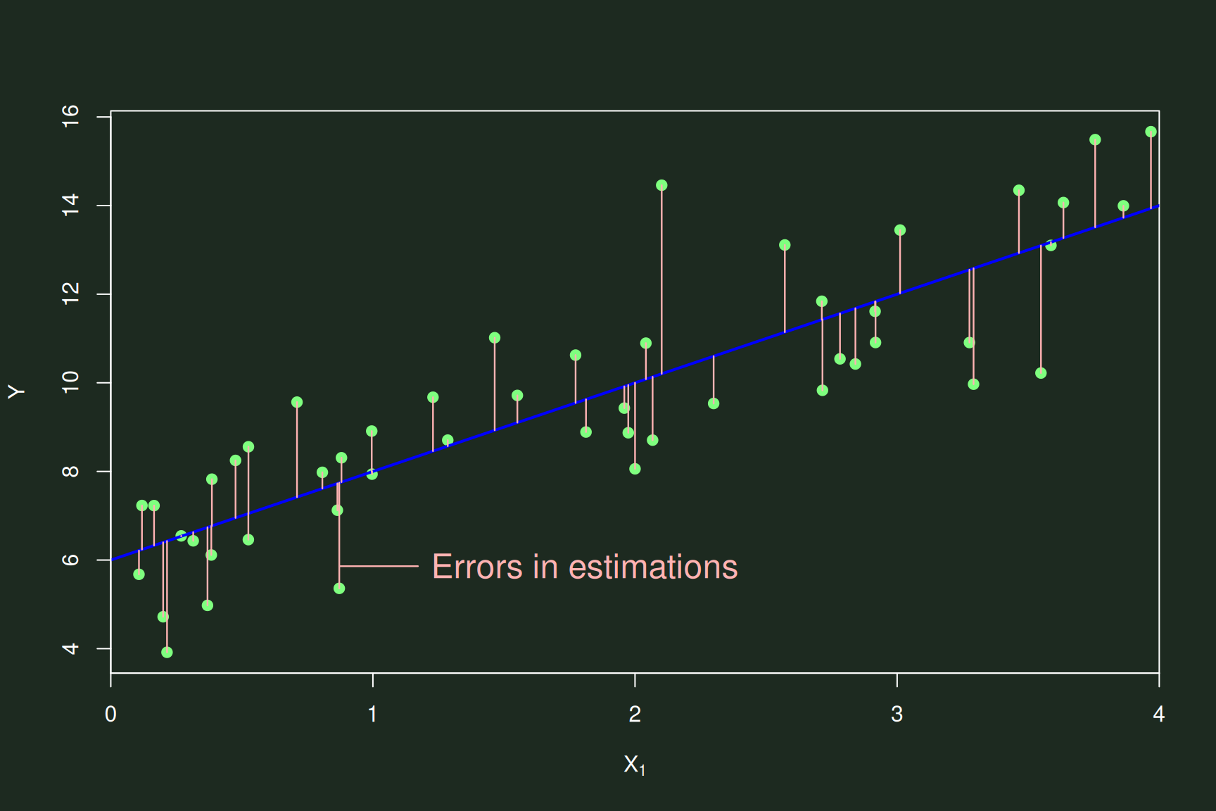
- Unexplained information—error in our model: \(e\)
- Significance tests the strength of the model’s “signal” against
error’s “noise”
- I.e., whether we can distinguish the signal from the noise
Signal-to-Noise in Linear
Models (cont.)
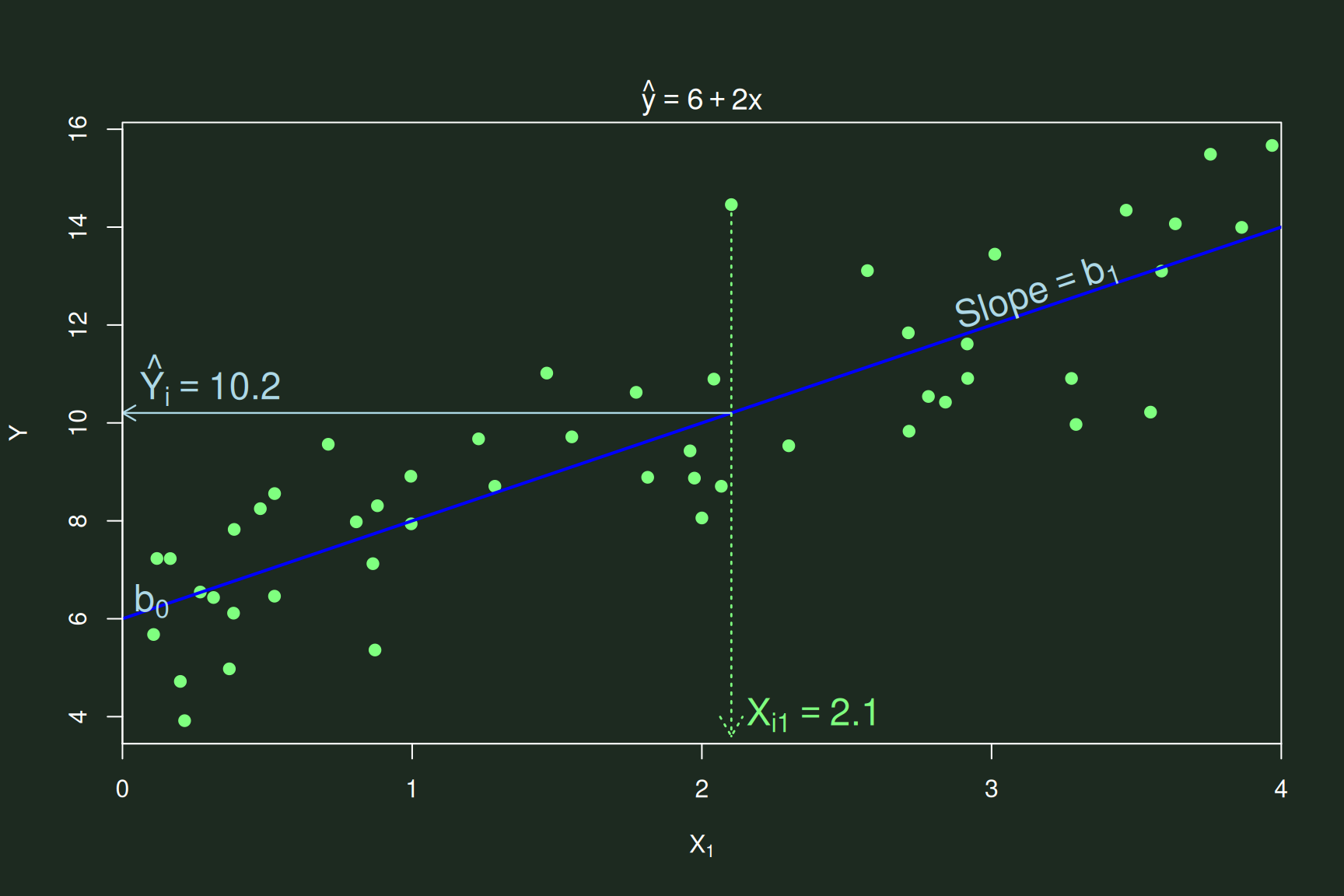
\(\hat{Y}_{i} = b_{0} + b_{1}X_{i1} +
e_{i}\)
- The sum of squares representation of this partition into predictors
& error looks like:
\[\sum\limits_{i=1}^{n} (Y_{i} -
\overline{Y})^{2} = \sum\limits_{i} (\hat{Y}_{i} - \overline{Y})^{2} +
\sum\limits_{i} ({Y}_{i} - \hat{Y}_{i})^{2}\]
Signal-to-Noise in Linear
Models (cont.)
\(\sum\limits_{i=1}^{n} (Y_{i} -
\overline{Y})^{2} = \sum\limits_{i} (\hat{Y}_{i} - \overline{Y})^{2} +
\sum\limits_{i} ({Y}_{i} - \hat{Y}_{i})^{2}\)
- I.e.,the squared sum of the differences of each instance (\(Y_{i}\)) from the mean (\(\overline{Y}\)) equals:
- The squared sum differences of each predicted value (\(\hat{Y}_{i}\)) from the mean
- Plus the squared sums of differences of the actual values (\(Y_{i}\)s) from the respective predicted
values
Signal-to-Noise in Linear
Models (cont.)
- Another way of saying this:
\(\sum\limits_{i=1}^{n} (Y_{i} -
\overline{Y})^{2} = \sum\limits_{i} (\hat{Y}_{i} - \overline{Y})^{2} +
\sum\limits_{i} ({Y}_{i} - \hat{Y}_{i})^{2}\)
- Is to say this:
\(\text{Total SS = SS from Regression + SS
from Error}\)
- Or, further condensed as:
- \(SS_{Total} = SS_{Reg.} +
SS_{Error}\)
Signal-to-Noise in Linear
Models (end)
- Using \(SS_{Total} = SS_{Reg.} +
SS_{Error}\),
- We can compute the ratio of predicted to actual:
Ratio of Predicted-to-Actual Variance = \(\frac{SS_{Reg.}}{SS_{Total}}\)
- Or, equivalently as \(1 -
\frac{SS_{Reg.}}{SS_{Error}}\)
- We typically represent this ratio as
R²:
\[R^{2} = \frac{SS_{Reg.}}{SS_{Total}} = 1
- \frac{SS_{Reg.}}{SS_{Error}}\]
Yep, that’s what \(R^{2}\) means in
ANOVAs ☻
Adding More Terms to Models
- Adding another variable to the equation:
\(\hat{Y}_{i} = b_{0} + b_{1}X_{i1} +
b_{2}X_{i2} + e_{i}\)
- \(X_{i2}\) = Participant \(i\)’s value on the other variable (\(X_{2}\)) added to the model
- \(b_{2}\) = Slope for \(X_{2}\)
- Since there are multiple predictors (\(X\)s) in this model,
- This is called a multiple linear regression
More About the Equation (cont.)
- We can continue to add still more variables to the model, e.g.,
\(X_{3}\) and \(X_{3}\):
\[\hat{Y}_{i} = b_{0} + b_{1}X_{i1} +
b_{2}X_{i2} + b_{3}X_{i3} + b_{4}X_{i4} + e_{i}\]
- When there are a lot of terms in the model, then we usually
abbreviate the equation to:
\[\hat{Y}_{i} = b_{0} + b_{1}X_{i1} ... +
b_{k}X_{ik} + e_{i}\]
- Were \(k\) denotes the number of
variables
Adding More Terms to Models (cont.)
\(\hat{Y}_{i} = b_{0} + b_{1}X_{i1} ... +
b_{k}X_{ik} + e_{i}\)
- We can test interactions by adding additional terms
- E.g., \(... b_{1}X_{i1} + b_{2}X_{i2} +
\mathbf{b_{3}(X_{i1}X_{i2}}) ...\)
- Or test non-linear effects, also by adding terms
- E.g., \(... b_{1}X_{i1} +
\mathbf{b_{2}X_{i1}^{2}} ...\)
Adding More Terms to Models (end)
- Just as we separated out the effects of the predictors,
- We can separate out sources of error
- E.g., per predictor/term in the model
- We can also combine error terms
- E.g., we can “nest” one variable into another
- Patients nested within hosptital units
- Wave (time) nested within patient
Modeling Linear & Non-Linear Relationships
\(\hat{Y}_{i} = b_{0} + b_{1}X_{i1} ... +
b_{k}X_{ik} + e_{i}\)
- \(Y\) is assumed to follow a
certain distribution
- This determines how error is modeled
- E.g., is error usually assumed to be normally distributed
- But both distributions can be assumed to be something else
Modeling Linear & Non-Linear Relationships (cont.)
\(\hat{Y}_{i} = b_{0} + b_{1}X_{i1} ... +
b_{k}X_{ik} + e_{i}\):
- \(X\)s can be nominal, ordinal,
interval, or ratio
- This affects how those variables are modeled
- As well as the error related to them
- We could transform the terms on the right
- E.g., raise them to a power or take their log
Modeling Linear & Non-Linear Relationships (cont.)
\(\hat{Y}_{i} = b_{0} + b_{1}X_{i1} ... +
b_{k}X_{ik} + e_{i}\)
- For an ANOVA (and t-tests):
- \(Y\) is assumed to be normally
distributed
- The \(X\)s are nominal
- The model terms are not transformed
- Leaving their relationship with \(Y\) linear
- Technically, called an “identity transformation”
- Meaning they are multiplied by 1:
\(\hat{Y}_{i} = 1 \times (b_{0} + b_{1}X_{i1}
... b_{k}X_{ik} + e_{i})\)
Modeling Linear & Non-Linear Relationships (end)
- The terms can be transformed in other models
- This transformation is called a Link Function
- Since it “links” the terms on the right to the predicted value of
\(Y\) on the left
- E.g., logistic regression uses a logarithmic (\(e\)) link:
\(\hat{Y}_i = \frac{e^{b_{0} +
b_{1}X_{i1} + \cdots + b_{k}X_{ik}}}{1 + e^{b_{0} + b_{1}X_{i1} + \cdots
+ b_{k}X_{ik}}}\)
which is more often written as:
\(\ln\!\frac{\hat{Y}_i}{1-\hat{Y}_i} =
\;b_{0}+b_{1}X_{i1}+\cdots+b_{k}X_{ik}\)
Generalized Linear Models
- That family of models is referred to as generalized
linear models
- I.e., we can generalize that linear model into other types
of models
- ANOVAs, t-tests, and logistic regressions are types of
generalized linear models
- Generalized linear models typically use maximum
likelihood estimation (MLE) to compute terms
- The ordinary least squares of ANOVAs, etc. is itself a specific type
of MLE
Generalized Linear Models (cont.)
- N.b., confusingly, in addition to generalized linear
models,
- There are general linear models
- “General linear model” simply refers to models you
already know.
- I.e., those with:
- Normally-distributed,
iid variables &
- Identity link functions
- Like ANOVAs & multiple linear regressions
Generalized Linear Models (cont.)
- Assumptions of generalized linear models:
- Relationship between response and predictors must be expressible as
a linear function
- Cases must be independent of each other
- Or that relationship should be part of the model
Generalized Linear Models (end)
- Assumptions of generalized linear models (cont.):
- Predictors should not be too inter-correlated (lack of multicollinearity)
- Linear regression simply cannot get accurate measures of two effects
if they cannot be easily separated
- The random error & link functions should approximate their
actual functions