3 Exploratory Factor Analysis
3.1 The Concept of Factor Analysis
Factor analysis is a member of a rather large family of analyses that—among other things—uses ostensible variables to measure and analyze non-ostensible constructs, domains, or what are generally called factors. In this sense, a “factor” is that non-ostensible thing that determines whatever value ostensible variables take on. Factor is intentionally a very general term here that can encompass true constructs/domains, but is also simply whatever underlying thing is driving what we actually see.
It is not, however, intended to imply a factor in a statistical model, nor a “factor” in math (a multiplicative product or common divisor). So, please forget whatever definition you already have for the word “factor” and understand it here as simply that non-ostensible thing that drives one or more ostensible variables. (Indeed, one of the two main types of factor analysis, “exploratory factor analysis,” revolves around trying to figure out just what the underlying factors really are. I won’t discuss here the other main type of factor analysis, confirmatory factor analysis.)
3.1.1 Role of Correlation/Covariance Matrix in Factor Analysis
All factor analyses per se begin with the assumption that the more that ostensible variables correlate with each other, the more likely they are to measure the same, underlying (non-ostensible) factor. This assumption may not be true, but factor analyses1 assume it is. And what factor analysis does—in essence—is group variables together based on how well they correlate2; in fact, most statistical software can conduct a factor analysis on a correlation matrix of data alone: we don’t need to have access to the raw data (except to know the sample size). Given this, it may help to look at factor analysis first through the lens of a sample correlation matrix:
| Item 1 | Item 2 | Item 3 | Item 4 | |
|---|---|---|---|---|
| Item 1 | 1 | .80 | .10 | .20 |
| Item 2 | .80 | 1 | .05 | .15 |
| Item 3 | .10 | .05 | 1 | .90 |
| Item 4 | .20 | .15 | .90 | 1 |
In this correlation matrix, Items 1 and 2 are strongly correlated with each other, but neither correlates well with Items 3 or 4. Alternatively, Items 3 and 4 correlated well with each other (but not with Items 1 & 2). In this example, we wouldn’t be surprised if Items 1 and 2 measured the same thing and if this “thing” was largely unrelated to whatever Items 3 and 4 measured. In this example, then, we would expect that Items 1 and 2 are both ostensible manifestations of the same non-ostensible factor, and that Items 3 and 4 are the manifestations of an other non-ostensible factor.
With such a simple and clear example, we wouldn’t need to conduct a factor analysis: Our eyes can be trusted well enough here. Often, however, the picture is not as clear or simple, and we may yearn for some objective process firmly grounded in common, sensible assumptions and well-tested by research. For these occasions, we may turn to factor analysis.
3.1.2 Factor Analysis Is Similar to the Linear Regression Analyses You Already (Should) Know
As I noted above, factor analysis itself relies on the correlation matrix (or, similarly, the variance/covariance matrix3). There are different ways to analyze this matrix (or derive it and related statistics from the raw data), but in general, factor analysis conducts analyses conceptually similar to multivariate multiple regressions4 to determine how the items “load” onto the factors very similarly to how we estimate the \(beta\)- or b-weights for parameters in a linear regression. And like, e.g., an ANOVA, we not only get stats for how well our terms explain the data, we get stats (like Mean Square Error) for the extent to which our terms don’t fit the data. (More on this much later.)
3.2 Steps to Conducting an Exploratory Factor Analysis
(Please note that I broke out the steps here a bit differently than I did in the presentation. The steps are the same in both, I simply divided the same procedure into a different number of steps based on how well each worked for the two media. Costello and Osborne (2005) offer more good guidance.)
3.2.1 1. Estimate the Number of Factors
In multivariate analyses like a MANOVA, we know ahead of time how many DVs there are. Similarly, to get measures of how well the ostensible variables (e.g., items5) load onto the factor(s), we need first to get a sense of how may factors there may be. Therefore, the first step to an exploratory factor analysis (EFA) is to estimate the number of factors to use for further analysis.
The number of factors we choose could range from 1 to the number of items we have.
If we were to choose that the number of factors equaled the number of items (e.g., saying that there are 10 factors that underlie a 10-item instrument), we would essentially be saying that every item measures something different. This may be so, and would mean that there really isn’t any reason to conduct a factor analysis since it wouldn’t help us understand the data any better than item-level scores.
Often, though, when we conduct item-level analyses means we can’t easily (and unbiasedly) tease apart interesting from uninteresting variance—or we may find all variance “interesting” and never see the forest for for the trees. There are certainly times to scrutinize each item, but our ultimate goal is hopefully bigger—more profound—things than that.
Therefore, we strive to choose a smaller number of factors than items. But how much smaller? The general strategy is to find a number of factors that explains “enough” of the data. And so, a lot of thought has gone into what we mean by “enough.” One common criterion is to choose any factor that accounts for more of the data than an individual item does.
Another common criterion is to choose those factors that seem to “stand apart” from all of the other factors.
But all of this makes little sense without some underlying structure to guide it.
1.1. Drop-offs in Scree Plots
One of the earliest and biggest contributors to factor analysis was Raymond Cattell. An astoundingly productive and brilliant man, Cattell was also not above controversy for what were either his political beliefs or misunderstandings of them{^He may or may not have believed—as Galton certianly did—in eugenics and other right-wing supremacist positions throughout much of his life]. Whoever he was as a person, he was a gifted researcher, able indeed to see the “forest” and even to devise ways for us to do so better ourselves.
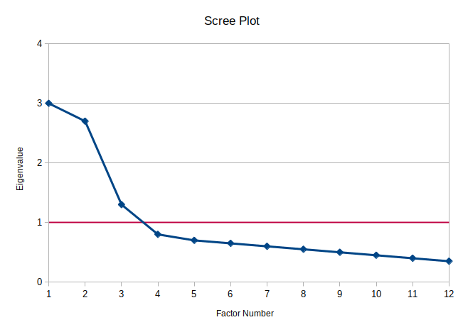
Perhaps his most lasting strategy was to use what he called “scree” plots to help decode how many factors to choose. “Scree” is the collection of rubble that gathers at the bottom of a cliff or plateau. The idea is that we’re interested in the solid, prominent cliff and not the rubble. We can choose whichever factors “stand out” above the scree of other factors. In the following plot, we may thus decide that this 12-item instrument contains two factors that account for most of the variance since the first two dots make what nearly looks like a ledge with all of the other ten dots fat below it—like rubble at the base of a cliff:
1.1. Eigenvalues Greater than 1
Meanings of “Eigenvalue”
Meaning 1: Proportion of Total Variance
The y-axis in the scree plot measures each factor’s eigenvalue. Eigenvalues, commonly used in mathematics and engineering, represent the amount of total variance explained by a given factor in the context of factor analysis.
Here’s how it works:
- The sum of all eigenvalues equals the total number of variables (or items) analyzed. For example, in a 12-item analysis, the eigenvalues in the scree plot will sum to 12.
- The eigenvalue for the first factor is 3. This means: \[ \frac{3}{12} = 0.25 \] Thus, the first factor accounts for 25% of the total variance.
If we compare this to correlations, the square root of this proportion (\(\sqrt{0.25} = 0.5\)) suggests an average correlation (\(r\)) of 0.5 between the items and the factor. This aligns with the principle that variance is the square of correlation.
For the first two factors (eigenvalues of 3 and 2.7), their combined contribution is: \[ \frac{3 + 2.7}{12} = \frac{5.7}{12} = 0.475 \] or nearly half of the total variance.
Meaning 2: Sum of Items’ Squared Loadings on a Factor
An eigenvalue can also be understood as the sum of the squared loadings of all items on a factor. To illustrate:
Suppose a 4-item instrument has the following factor loadings:
\[ \text{Factor}_1 = .7x_{1} + .5x_{2} + .1x_{3} + .2x_{4} \]
Here: - \(x_{1}\) through \(x_{4}\) are scores on the items in the instrument. - Factor loadings (0.7, 0.5, etc.): The correlations between the items and the factor.
The eigenvalue for the factor is calculated as the sum of the squared loadings:
\[ .7^{2} + .5^{2} + .1^{2} + .2^{2} = .49 + .25 + .01 + .04 = .79 \]
Thus, the eigenvalue is 0.79. This represents the total variance accounted for by the factor across these four items.
For the 12-item scree plot example, the eigenvalue for the first factor is 3. This implies that the sum of the squared loadings of the 12 items onto the first factor equals 3.
Why squared loadings?
- Factor loadings are essentially correlations, and squaring them converts correlations into proportions of explained variance. Since an eigenvalue represents the proportion of total variance accounted for by a factor, it must be based on the squared loadings.
Meaning 3: Relative Contributions of Individual Items
As noted earlier, the sum of all eigenvalues equals the total number of items. In the 12-item example, the eigenvalues sum to 12. This is because, by definition, the eigenvalue for any single item (if treated as a factor) equals 1.
- Implication: A factor with an eigenvalue greater than 1 accounts for more variance than any single item.
- Conversely, a factor with an eigenvalue less than 1 contributes less variance than a single item.
This is why a common criterion for factor retention is Kaiser’s Criterion, which retains only factors with eigenvalues greater than 1. Looking at the scree plot:
- Factors with eigenvalues less than 1 (e.g., Factors 4 through 12) do not contribute enough variance to justify their inclusion.
- Retaining such factors would mean adding complexity without meaningful additional information.
Takeaway: If a factor has an eigenvalue less than 1, it is generally better to rely on the individual items rather than attempting to interpret that factor.
1.3. Theory (or Practicality)
I purposely made Factor 3 in that scree plot above just a little greater than 1 (it’s 1.3). Since it’s greater than 1, we may want to keep it. Since it’s much lower than the next-larger factor (Factor 2), we may want to exclude it. We could use either criterion to justify our decision, so how do we decide?
Factor analysis—especially exploratory factor analysis—is not entirely an objective task. We should thus not simply swallow whole the results of factor analysis; we should chew on it and see if it tastes like something real. In this case, we could look at the results we get from choosing a 2-factor solution with those of a 3-factor solution and decide ourselves which appears to make more theoretical or practical sense.
3.2.2 2. Evaluate the Results
The second conceptual step in exploratory factor analysis is to evaluate the results we obtain given the number of factors we chose. And yes, it’s often worth playing around here, choosing different numbers of factors, and maybe even selecting subsets of items (as I did with when I removed the items from the APT that compared animals to humans).
In exploratory factor analysis, the main way we evaluate the results is by reviewing how well various items load onto the various factors. We review them to see if the factors make sense, if they provide any good insights, etc.
Often when we review how well the items load onto the factors, we will find that items load pretty well onto more than one factor. To turn again to the 4-item example I gave in the presentation, the items had the following loadings onto the two factors:
Factor1 = .7x1 + .5x2 + .1x3 + .2x4
Factor2 = .1x1 + .1x2 + .6x3 + .8x4
Sure, the loadings of .1 are really small. But what about that item 4 that loaded a bit onto both factors?
One criterion is to simply choose the highest loading (putting item 4 onto Factor 2). Another is to place items onto any and all factors on which its loading is >.3.
Note that an item may not load well onto any factor. (Again, commonly this means that its loadings are all less than .3 on all factors.) Such items deserve especial attention—and may well be removed from all factors (and possibly even instrument scores and other analyses).
3.2.3 3. Review Different “Rotations” of the Factors
As I wrote just above, the four items load a bit onto both factors. Since all four item scores would be part of both factors’ scores, these two factors themselves would be slightly correlated. When factors are allowed to be correlated like this, we say they are “oblique” to each other; they are called oblique because if I plotted them as two axes, those axes would be at right angles to each; the term for two lines (axes) that are neither perpendicular nor parallel is “oblique.”
Why go through all the trouble of calling them oblique when we could just say they’re correlated? Because we can do further mathemagic on the factors and force them to be uncorrelated—and this involves “rotating” the axes so that they are indeed perpendicular to each other. Of course, even that is not eldritch enough, so instead of saying the factors are now perpendicular, we say they’re “orthogonal,” which means the same thing.
To make matter even worse, there are different ways to rotate factors into orthogonality—and even different ways to rotate them to be variously oblique. The relative merits of the growing number of rotation techniques is a vibrant area of research, with no clear winner found.
Choosing Which Rotations to Use
In general, it’s good advise to try out at least one orthogonal and one oblique rotation and see how this helps us interpret the data.
Orthogonal Rotations
Orthogonal rotations force all factors to be unrelated to each other. These rotations therefore use various procedures to maximize the differences between factors.
Varimax is by far the most popular orthogonal rotation method, and it is often the default choice when there is no strong preference for another method. Its primary goal is to simplify the interpretation of factors by redistributing the variance of loadings to make high loadings higher and low loadings lower. Specifically, it maximizes the variance of the squared loadings for each factor across all items. In practice, this results in a factor structure where each factor has a few strongly loading items and many items with near-zero loadings. This simplification helps make the factors more interpretable. Varimax does not inherently make factor eigenvalues more similar or the proportion of explained variance more equal among factors, though it can result in a more balanced distribution in some cases.
Quartimax is another common orthogonal rotation method. While varimax aims to simplify the interpretation of factors, quartimax focuses on simplifying the interpretation of items. It does this by maximizing the variance of squared loadings for each item across all factors. In practice, quartimax tends to produce a factor structure where items load strongly on a single factor while having minimal loadings on others. This can make it easier to identify which items belong to which factor. However, quartimax often results in a factor structure where the first factor dominates, accounting for the largest proportion of the total variance. This makes the factors less balanced in terms of variance explained. For example, applying quartimax to the first two factors in a scree plot would likely accentuate the difference in eigenvalues between those factors, making the first factor seem more dominant.
There are plenty of other orthogonal rotations, but both of these have stood the test of time (and even some formal scientific tests) and should work well enough for most data.
Oblique Rotations
There are even more oblique rotations. They also tend to require a bit more hands-on involvement from the researcher. Luckily, though, for the two I describe next, this just means deciding the maximum possible value for how strongly the factors can correlated with each other. In other words, I could determine ahead of time that I want my factors to have correlation coefficients with each other that are no larger than .4.
- Promax is a common oblique rotation that in fact begins with an orthogonal rotation before “relaxing” this orthogonality requirement enough to let factors correlate with each other (either to a least-squares sense or to the maximum level you set ahead of time.) It tends to give rather easily-interpreted loadings onto the factors.
- Direct Oblimin doesn’t begin with an orthogonal rotation like promax but instead attempts to find the best axis for each factor and then modifies this slightly to try to reduce how much items load onto each factor.
Promax will tend to produce factors that are more orthogonal than direct oblimin.
3.2.4 3. Interpretation
This is arguably not a single, discrete step. Instead, one should be considering what is happening at each of the other steps, reflecting upon how it relates to apposite theories, and using one’s own judgment to guide analyses.
Nonetheless, researchers do tend to step back at the end of one round of factor analysis to consider how things look. I, too, recommend making sure there is at least this one deliberate pause to reflect on what the results imply about data and their larger meanings.
Similarly, you may now want to stop to think about all that I’ve written here—and let me know what questions you have.

Other analyses related to factor analysis don’t necessarily make this assumption, and this assumption can be relaxed with, e.g., confirmatory factor analysis. Nonetheless, it may help to understand the basics by going with this otherwise common assumption.↩︎
Remind you of the classical measurement theory’s concept of reliability?↩︎
A variance/covariance matrix—also simply called a covariance matrix for short—is simply a correlation matrix before the values in it are standardized. (Remember, correlations are measures of shared variance—that are standardized to values between 0 and 1 (and designated as positive or negative depending on the direction of the values).)↩︎
“Multivariate” here means that there are more than one criteria (“DVs”) and “multiple” means there’s more than one predictors (“IVs”); the criteria here are the non-ostensible factors we’re estimating, and the predictors are the ostensible variables (e.g., items).↩︎
So far, I’ve talked about the items that are analyzed for their inter-correlations. However, we could include any ostensible variable—not just the items of an instrument. We could include demographic variables, scores on other measures, or even predictors (IVs) and criteria (DVs). When we include predictors and criteria in our “factor analyses,” we are simply starting to turn them into structural equation models.↩︎